Excel: Use Conditional Formatting to format cells by formula
Categories: Development Notes; Tagged with: Excel; @ May 15th, 2014 23:31Requirement:
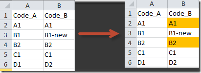
As a (junior) Excel user, I want to compare two columns and change the background colour for the cells which is not consistent.
Steps:
1. Create New Rule:
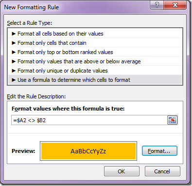
you may select the B2, and click Conditional Formatting > New Rule:
Configure the formula and the format.
2. Apply the the rule:
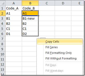
You may right click the ‘+’and then drug, select the ‘Fill formatting Only’ when drop.
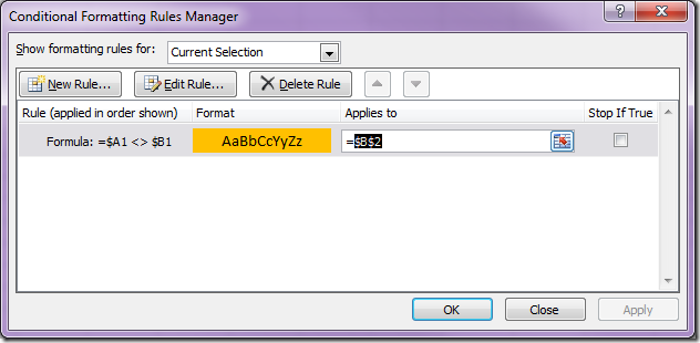
Or you can use Conditional Formatting > Manage Rules:
to change the “Applies to…” and then “Apply”
Excel 首字母大写
Categories: Development Notes • 分享; Tagged with: Excel; @ November 28th, 2012 20:38使用Proper函数只能做到每个单词的首字母大写, 该单词的其余字母会变小写。
但如果有时只需要将首字母大写,剩余字符保持不变, 此种情况下可使用公式操作:
= UPPER(LEFT(A2))&RIGHT(A2,LEN(A2)-1)
Excel: count nonblank column numbers using COUNTA 使用COUNTA计算Excel非空行数
Categories: Development Notes; Tagged with: Excel; @ September 19th, 2012 19:16Use COUNTA function:
Counts the number of cells that are not empty and the values within the list of arguments. Use COUNTA to count the number of cells that contain data in a range or array.
>>COUNTA function Details<<
Adding drop down list in Excel 在Excel中增加下拉框
Categories: Development Notes; Tagged with: Excel; @ September 5th, 2012 17:331. preparing the data source: just input your values in file;
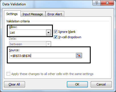
2. Edit the validation of the target cell(s): Data/Validation:
3. Click ‘OK’, now, you can see the list when you click the cell. if needed, you can use the auto fill tool to set validation for other cells.
Excel: Get cell comments
Categories: Development Notes; Tagged with: Excel; @ August 23rd, 2012 19:051. Alt + F11, in the opening window, click: Insert>Module, paste the folling code:
Function getComment(incell) As String

On Error Resume Next

getComment = incell.Comment.Text

End Function
2. Alt + Q to quit the window
3. use the funciton in cell, like:
=getComment(A1) , will fill the cell with A1’s comments
